Question and Answers Forum

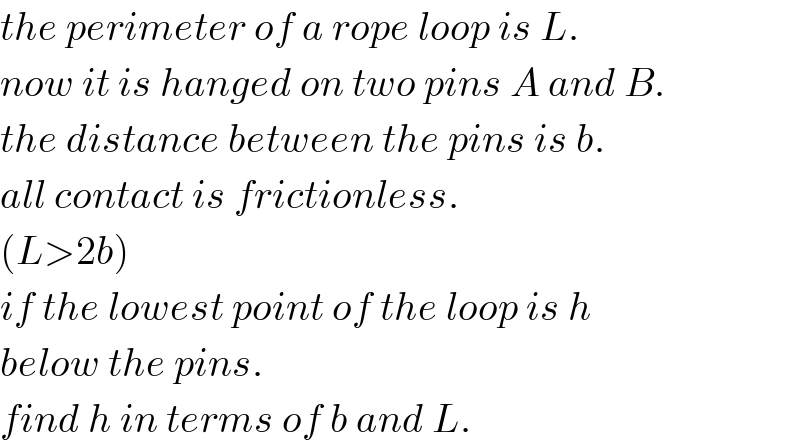
Question Number 66527 by mr W last updated on 16/Aug/19

Commented by mr W last updated on 16/Aug/19
Answered by mr W last updated on 17/Aug/19

Commented by mr W last updated on 17/Aug/19

Commented by mr W last updated on 17/Aug/19
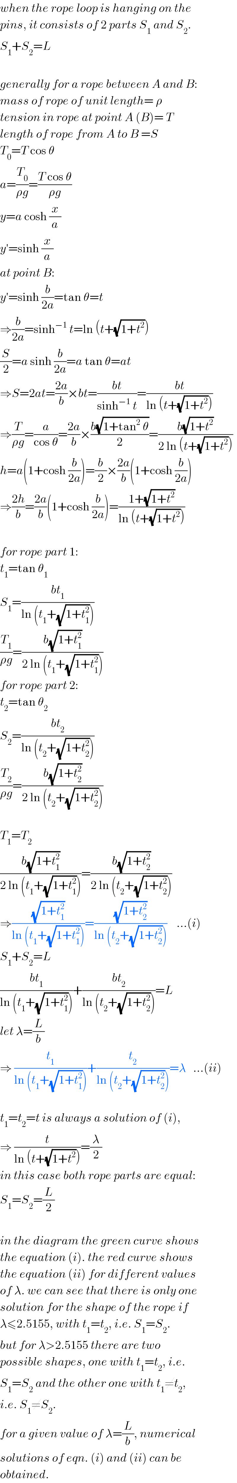
Commented by mr W last updated on 17/Aug/19

Commented by mr W last updated on 17/Aug/19

Commented by Cmr 237 last updated on 17/Aug/19

Commented by mr W last updated on 17/Aug/19